
Share


BigQuery costs are comprised of storage (active and lon
g term ), analysis (querying) and streaming inserts. Unfortunately, the built-in
Google Cloud Platform
billing dashboard doesn’t allow you to break down the costs by anything other than pricing SKU. Therefore, if you wanted to know the biggest contributor to your monthly storage costs, or which user runs the most expensive queries, it’s not possible with the out-of-the-box reporting. However, with a simple dynamic SQL statement querying the information catalog, the answer is possible. Let’s start with BigQuery storage costs.
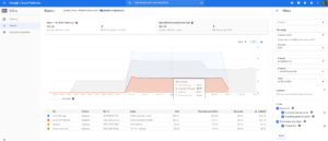 The lowest level of billing details available in Google Cloud Platform are the pricing SKUs. Costs by dataset or table are not possible out of the box.[/caption]
BigQuery storage is priced in two tiers: active and long-term. Once your data is loaded into BigQuery, you’re charged for storing it as active storage. Storage pricing is based on the amount of data stored in your tables when it’s uncompressed. The size of the data is
calculated
based on the data types of the individual columns and the amount of data stored in the columns. Active storage charges $0.02/GB after the first 10 GB.
If a table or partition is not edited for 90 consecutive days, the price of storage for that data automatically drops by approximately 50 percent to $0.01/GB when it’s automatically moved into long term storage. There is no degradation of performance, durability, availability or any other functionality, just the price discount.
If you edit the table (or partition), the price reverts back to the active storage pricing, and the 90-day timer starts counting from zero. Anything that modifies the data in a table resets the timer, including:
The lowest level of billing details available in Google Cloud Platform are the pricing SKUs. Costs by dataset or table are not possible out of the box.[/caption]
BigQuery storage is priced in two tiers: active and long-term. Once your data is loaded into BigQuery, you’re charged for storing it as active storage. Storage pricing is based on the amount of data stored in your tables when it’s uncompressed. The size of the data is
calculated
based on the data types of the individual columns and the amount of data stored in the columns. Active storage charges $0.02/GB after the first 10 GB.
If a table or partition is not edited for 90 consecutive days, the price of storage for that data automatically drops by approximately 50 percent to $0.01/GB when it’s automatically moved into long term storage. There is no degradation of performance, durability, availability or any other functionality, just the price discount.
If you edit the table (or partition), the price reverts back to the active storage pricing, and the 90-day timer starts counting from zero. Anything that modifies the data in a table resets the timer, including:
 Query executed using EXECUTE IMMEDIATE scripting function executes in two stages but appears to the user as executing as one.[/caption]
 The dynamic SQL query (sampled) produce in stage 1.[/caption]
 The first 10 results after stage 2 execution completed.[/caption]
The results above display the storage costs by each individual dataset and table. With these results, spotting costly data is easy. Subsequently, you can optimize the storage costs by removing unused tables or datasets. In another post, we’ll discuss getting analysis costs by user and table to see where optimizations can be made in that area. Stay tuned!
Questions? Feel free to
contact us.
The first 10 results after stage 2 execution completed.[/caption]
The results above display the storage costs by each individual dataset and table. With these results, spotting costly data is easy. Subsequently, you can optimize the storage costs by removing unused tables or datasets. In another post, we’ll discuss getting analysis costs by user and table to see where optimizations can be made in that area. Stay tuned!
Questions? Feel free to
contact us.
Google Cloud Platform BigQuery Costs
[caption id="attachment_39453" align="alignnone" width="993"]
The lowest level of billing details available in Google Cloud Platform are the pricing SKUs. Costs by dataset or table are not possible out of the box.[/caption]
BigQuery storage is priced in two tiers: active and long-term. Once your data is loaded into BigQuery, you’re charged for storing it as active storage. Storage pricing is based on the amount of data stored in your tables when it’s uncompressed. The size of the data is
calculated
based on the data types of the individual columns and the amount of data stored in the columns. Active storage charges $0.02/GB after the first 10 GB.
If a table or partition is not edited for 90 consecutive days, the price of storage for that data automatically drops by approximately 50 percent to $0.01/GB when it’s automatically moved into long term storage. There is no degradation of performance, durability, availability or any other functionality, just the price discount.
If you edit the table (or partition), the price reverts back to the active storage pricing, and the 90-day timer starts counting from zero. Anything that modifies the data in a table resets the timer, including:
- Loading data into a table (or partition)
- Copying data into a table (or partition)
- Writing query results to a table (or partition)
- Using the Data Manipulation Language (DML)
- Using Data Definition Language (DDL)
- Streaming data into the table (or partition)
EXECUTE IMMEDIATE scripting function
Regardless of which pricing class your data falls into, often you want a breakdown of which tables (or datasets) in your project are storing the most rows or data and thus costing the most. This information has always been available in the information catalog within BigQuery. Previously, you would have to execute at least two separate queries, but with the recent introduction of the EXECUTE IMMEDIATE BigQuery scripting function, it’s now possible to analyze all the tables and datasets across your projects and summarize the data costs in one single dynamic SQL query. [caption id="attachment_39455" align="alignnone" width="969"]
Query executed using EXECUTE IMMEDIATE scripting function executes in two stages but appears to the user as executing as one.[/caption]
Query Breakdown
Let’s break down this query’s execution. The first step is to create a dynamic SQL statement. This step ensures it’s valid before passing it to the next step. The second step executes it as it would any other SQL query. The three components of the above query are described below. Schemas subquery (shown below) selects each dataset in the executing project in the first column and another column showing the last dataset when ordered ascending A-Z. The subquery is required to extract all the possible datasets in the project to be used as variable to substitute into that many SQL statements querying the __TABLEs__ metadata table from each corresponding dataset. SELECT schema_name, LAST_VALUE(schema_name) OVER (PARTITION BY catalog_name ORDER BY schema_name ASC ROWS BETWEEN UNBOUNDED PRECEDING AND UNBOUNDED FOLLOWING) AS last_schema FROM INFORMATION_SCHEMA.SCHEMATA Static subquery (shown below) is a query selecting string constants used to create the bulk of the dynamic SQL statement. The %s will be used in the final query to substitute the rows representing all the datasets in the project. It’s possible to combine STATIC and SCHEMAS sub-select statements into one, but they’re separated here to help with simplicity. SELECT " SELECT project_id, dataset_id, table_id, sum(row_count) as row_count, round(SUM(size_bytes)/1000000000,0) AS GB FROM `%s.__TABLES__` group by 1,2,3" AS SQL, " union all " AS cmd_u, " order by 1, 5 desc " AS cmd_f Final query (shown below) cross joins both sub-select statements defined above and substitutes the dataset into the static SQL statement with a “union all” for most, except the last one, in which an “order by” clause is used at the close of the dynamic SQL statement. SELECT ARRAY_TO_STRING(ARRAY_AGG(sql_command_rows),"") AS generated_sql_statement FROM ( SELECT CASE WHEN schemas.schema_name != schemas.last_schema THEN CONCAT(FORMAT(static.sql,schema_name),static.cmd_u) ELSE CONCAT(FORMAT(static.sql,schema_name),static.cmd_f) END AS sql_command_rows FROM static CROSS JOIN schemas ORDER BY schema_name ASCStage 1
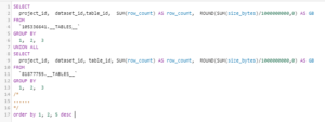
The first-stage results from the query are shown in the screenshot below (sampled). It’s a large union of all tables within all datasets in the executing project and sums the row and storage bytes. Before the introduction of the EXECUTE IMMEDIATE function, you would have had to take these results and execute them in a separate query. [caption id="attachment_39457" align="alignnone" width="977"]
The dynamic SQL query (sampled) produce in stage 1.[/caption]
Stage 2
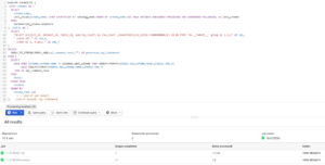
Executing the dynamic SQL statement produced in stage one produces a row for each table, by dataset and project, and the row counts and total size (GB). From these results, a simple pivot will allow aggregated totals by either project or dataset. [caption id="attachment_39456" align="alignnone" width="967"]
The first 10 results after stage 2 execution completed.[/caption]
The results above display the storage costs by each individual dataset and table. With these results, spotting costly data is easy. Subsequently, you can optimize the storage costs by removing unused tables or datasets. In another post, we’ll discuss getting analysis costs by user and table to see where optimizations can be made in that area. Stay tuned!
Questions? Feel free to
contact us.