
Share


BigQuery MachineLearning (BQML) can train and serve ML models using only SQL to power marketing automation and help deliver personalized experiences.
Article Series Overview
In the “Use BQML to Activate Audiences on Google Marketing Platform (GMP)” article series, we’ll use unsupervised machine learning methods to build clusters of users grouped by their similarities to each other. We’ll analyze these clusters to extract insights and add meaning business labels to better understand them. Then we’ll load these clusters into Google Analytics using the Management API to turn them into segments and finally, we’ll build GA Audiences to activate these users across the GMP. Be sure to r ead our introduction article for insights into the technologies we’ll use and the business challenges we’re solving. This article covers data preparation.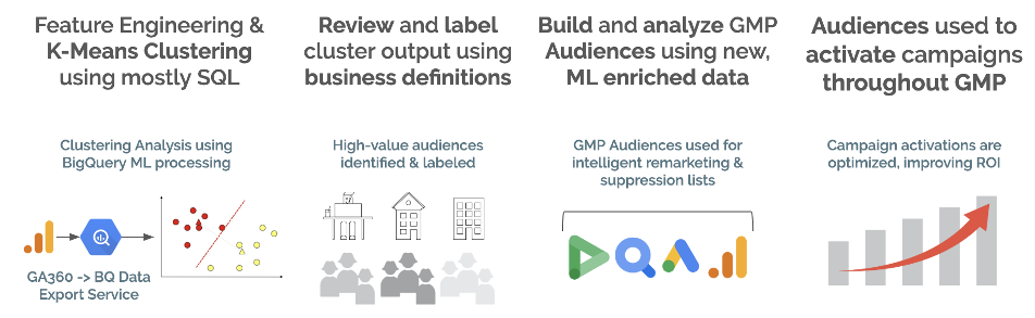
Data Preparation
We’ll use the Google Analytics Sample data in BigQuery for this demo. Using the Adswerve Data Layer Inspector+ tool, we take note of the important metadata being sent to Google Analytics. In this example, we see that clicking on a product sends a GA Enhanced Ecommerce event with the action set to “Quickview Click”. These labels will come in handy when we write our SQL.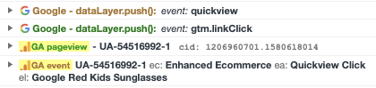 Once you’ve identified all the relevant events, you’ll want to take a look at the content taxonomy. Google provides access to its
Google Merchandise Demo GA Account, which can be helpful to acquire domain knowledge of the data and the quality. They expose the dates 8/1/2016 - 8/1/2017 within BigQuery,
so be sure to also use those in GA.
Next, we’ll want to perform Exploratory Data Analysis (“EDA”) on the data quality. These models can be sensitive to outliers, so it is a good practice to cull the data of anomalous records. K-Means clustering itself is a great tool to use analyze large sets of data and is helpful for outlier detection.
Once you’ve identified all the relevant events, you’ll want to take a look at the content taxonomy. Google provides access to its
Google Merchandise Demo GA Account, which can be helpful to acquire domain knowledge of the data and the quality. They expose the dates 8/1/2016 - 8/1/2017 within BigQuery,
so be sure to also use those in GA.
Next, we’ll want to perform Exploratory Data Analysis (“EDA”) on the data quality. These models can be sensitive to outliers, so it is a good practice to cull the data of anomalous records. K-Means clustering itself is a great tool to use analyze large sets of data and is helpful for outlier detection.
Google Colaboratory for Exploratory Data Analysis
I’ve shared a Google Colab document that can help bootstrap your EDA and data validation. Using Colaboratory, you can easily and securely share work within your company and iterate on versions to fine-tune analysis. In the example, we feed features like ‘day of week’, ‘row count’, ‘creation time’, and ‘table size (MBs)’ into a kmeans model and examine the results: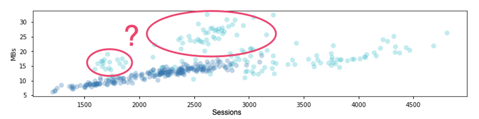
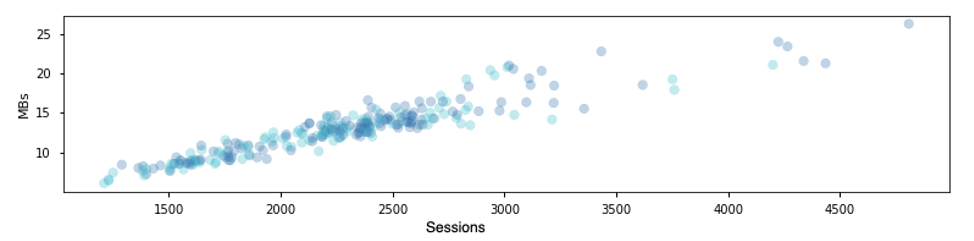
 In this example, we see that data collected previous to 11/24/2016 (1.48e9 epoch seconds) had tables with much higher MB per row. Normally, table size would be directly correlated with daily sessions, which holds true if we cull away data prior to the 1.48e9 epoch:
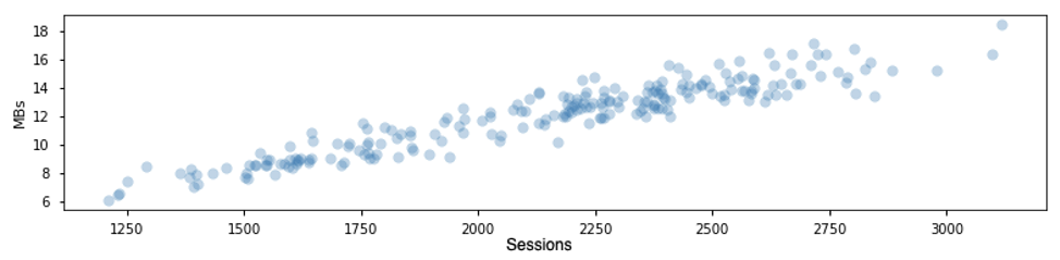
 Rather than culling the date, we could cull the cluster label that correctly identified the anomalous traffic. When we do this notice the x-axis change scale, down from +5000:
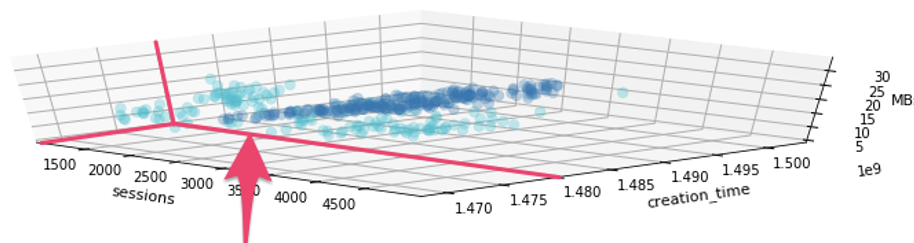
 In this case, high daily sessions are not considered anomalous and so we’ll stick to slicing the data by date rather than cluster label. Note below that the clustering model found the weekly-seasonal patterns in site performance:
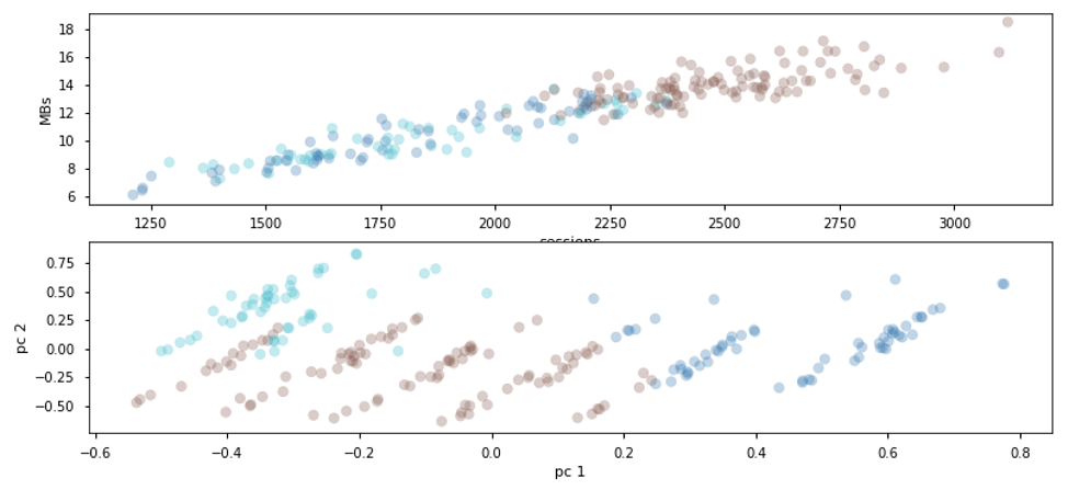 The brown labels show Monday - Thursday visits, dark-blue shows Friday - Saturday, while light-blue shows Sunday traffic. We see that peak traffic occurs Monday-Thurs when daily sessions are greater than 2,200. The inverse is true for weekend traffic + Friday. It’s likely that these audiences have different behavior patterns and require different marketing strategies.
Cloud Dataprep
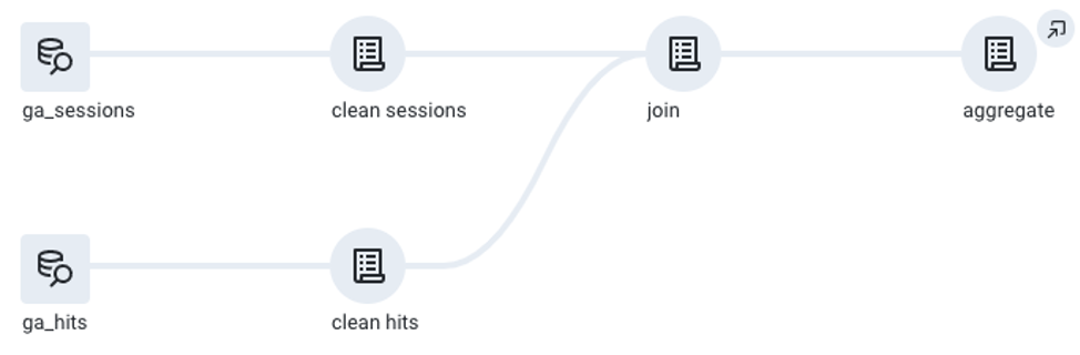
Cloud Dataprep can help you build a data pipeline from GA Export tables into cleaned and aggregated tables, ready for ML processing. There are many ways to build a pipeline, ie. using BQ views + BQ scheduled jobs, but Dataprep writes difficult and time-consuming SQL code so we don’t have to! Here is the SQL I begin with to feed by Dataprep pipeline:GA Sessions Query
SELECT

  date, visitStartTime, visitNumber, totals.*,

  trafficSource.*, device.*, geoNetwork.*,

  fullVisitorId, visitid, channelGrouping,

  concat(fullVisitorId, visitid) as sessionId

FROM `bigquery-public-data.google_analytics_sample.ga_sessions_20170801` -- ga_sessions_* when ready for full dataset
This is a simple way to access the session-scoped dimensions and metrics available in BigQuery. We write a similar query against the hits object ( learn more about BQ queries here ). The ga_sessions and ga_hits table have a common key between the two: sessionId. We generated this field by concatenating the fullVisitorId and visitId fields in our SQL, shown above. In the end, Datprep provides a pipeline that begins with raw ga_sessions and ga_hits tables, cleans them, joins them together and finally, aggregates the data on fullVisitorId.
Cleaning the Raw Data in Dataprep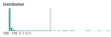
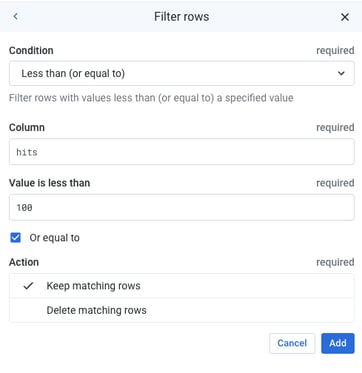 Cleaning the data consists of identifying anomalies and setting boundaries to make sure that your model is as generalized as possible, and not influenced by the outliers.
Setting an arbitrary value using a simple inspection of the histogram is sufficient. However, for production, you might want to add a bit more rigor to your decision boundaries.
Dataprep gives you many ways to clean and restructure your data and provides a pipeline that can be executed on new data.
The ability to export your “recipe” into a Dataflow job that can run on a schedule or on-demand is valuable. The recipe works on new data, allowing your audience model to continuously bring value to your organization.
Cleaning the data consists of identifying anomalies and setting boundaries to make sure that your model is as generalized as possible, and not influenced by the outliers.
Setting an arbitrary value using a simple inspection of the histogram is sufficient. However, for production, you might want to add a bit more rigor to your decision boundaries.
Dataprep gives you many ways to clean and restructure your data and provides a pipeline that can be executed on new data.
The ability to export your “recipe” into a Dataflow job that can run on a schedule or on-demand is valuable. The recipe works on new data, allowing your audience model to continuously bring value to your organization.
Joining ga_hits with ga_sessions using the synthetic sessionId field
After cleaning our raw ga_hits and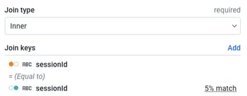 ga_sessions tables we want to join these two tables together using the synthetic “sessionId” field we created in our source queries:
concat(fullVisitorId, visitid) as sessionId
Dataprep gives us lots of options when joining datasets together. In this case, we use a simple inner join.
Sampling Data in Dataprep
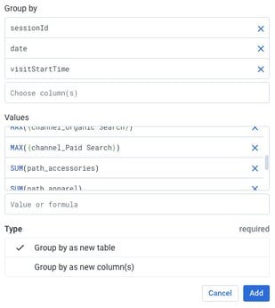
Dataprep pulls a sample to begin working with the data. It is always a good idea to run a random sample, or in this scenario, a cluster-based sample using sessionId. When cleaning data, I like to add favorable conditions to my cluster logic to ensure I’m not removing data that is representative of my “ideal” audience, ie. sessionQualityDim > 0Aggregating Session + Hit Data
Uploading Cluster Input Data
We now have cleaned data that has been prepared for ML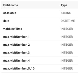 processing. Our final data preparation step
will be to add a publishing action to our Dataprep job.
We can choose BigQuery as a target for our job and can select to append, drop or truncate existing tables each run. We can even add a schedule to our job. You can envision a process that runs daily, looking for new data to prepare for machine learning.
Stay tuned for the part 3 in our “Use BQML to Activate Audiences on Google Marketing Platform (GMP)” series, “Modeling.” In the meantime, please
contact us
with any questions.
processing. Our final data preparation step
will be to add a publishing action to our Dataprep job.
We can choose BigQuery as a target for our job and can select to append, drop or truncate existing tables each run. We can even add a schedule to our job. You can envision a process that runs daily, looking for new data to prepare for machine learning.
Stay tuned for the part 3 in our “Use BQML to Activate Audiences on Google Marketing Platform (GMP)” series, “Modeling.” In the meantime, please
contact us
with any questions.