
Google announced unstructured data analysis is available directly within BigQuery ML. This announcement means we can feed images, videos and documents into machine learning models that allow us to perform detailed analyses. The fact this is available in BigQuery means this is all done using SQL—a feat previously only available with advanced coding skills using ML frameworks like Tensorflow.
In this article, we'll look at how Adswerve applied this new capability for Twiddy & Co, the leading vacation rental provider in the outer banks. Their visual content is critical for guests to find the vacation of their dreams. This project took Twiddy's in-house SQL skills and applied that to state-of-the-art machine-learning image analysis.
BQML Unstructured Data Overview
A picture is worth a thousand words and many more data points. Unstructured data analysis unlocks information hidden within complex objects – including images, audio, videos and documents. Currently, this capability is difficult and scarce. It’s also cutting edge, which comes with positives and negatives.
BigQuery has been able to serve custom Tensorflow models for years. However, the input was always tabular. For the first time, this capability is available with unstructured inputs. Using BigLake to mount to GCS, we have new Object Tables that can query the unstructured file's data and metadata.
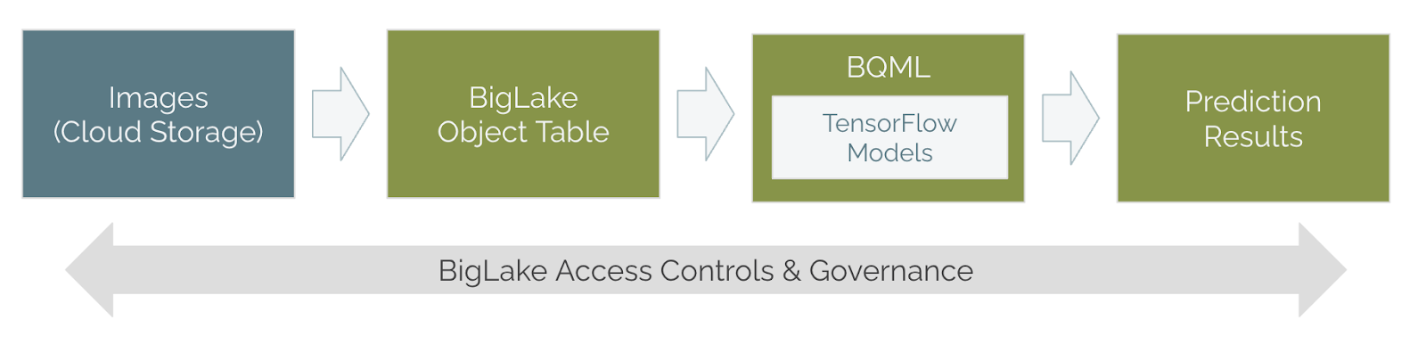
Security and governance come included. BigLake plugs into Dataplex for management at scale. Additionally, you inherit BigQuery access management, including row-level security.
Framing the Machine Learning Problem
There is much to say on this topic. Still, for this article, we'll keep it very brief:
Unstructured data analysis is great fun when you’re using baseline models, but pre-trained models only get you so far: given an input, they output prediction. In our case, that’s vacation rentals' featured images. We can and will analyze these outputs, but we need a model that improves the customer experience. To do this, we enhance the experience by selecting the best featured image. This is the challenge before us.
We built a SQL pipeline to deliver this capability. This is a great new skill for the many SQL analysts at Twiddy, and Adswerve is excited to share how we did it and what comes next.
Example Prediction Pipeline
For our example, we're going to run an image through a baseline image classification model. We’ll serve the model within BQML, and we'll use ML.PREDICT() to run inference against image data in the Object Table and retrieve image labels and feature vectors from machine learning models.
Prerequisite: Load images to a Cloud Storage bucket
To get started, we'll upload some images from our website CDN to Google Cloud Storage using the gsutil command line tool. You can install this locally on your computer with the Google Cloud SDK or access it remotely using Colab or Cloud Shell:
> gsutil cp /CDN/www/images/*.jpg gs://bqml-demo/images
Here are a handful of the images we'll be using later on in our prediction pipeline:
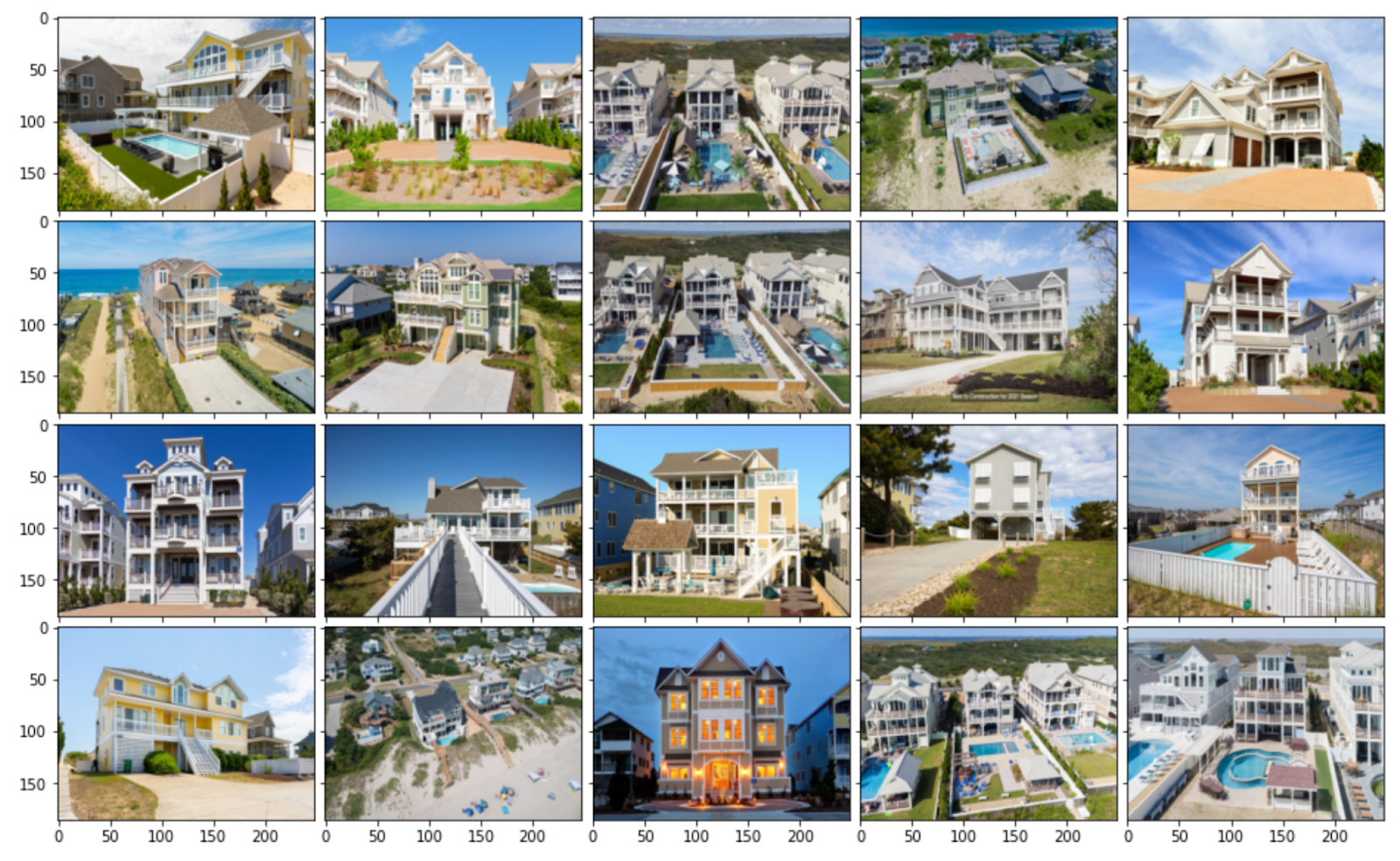
Note that because we're using Google Cloud Storage ("GCS") and BigQuery ("BQ"), the scale of the problem you bring to the table is effectively limitless. In our simple "proof of concept" pipeline, we processed over 52,000 images at ~20GB on disk—a drop in the Niagara Falls that is Google capacity.
Step 1: Create BigLake Object Table
This is a three-step process. First, we'll use the bq command line tool to create a BigLake Connection:
> bq mk --connection --location=US --project_id=bqml-demo
--connection_type=CLOUD_RESOURCE image-connection
The connection is an important piece of the BigLake architecture. It allows the two systems to communicate securely and gives teams governance by automatically creating a service account for CLOUD_RESOURCE connections. We’ll access this service account with bq show:
> bq show --location=US --project_id=bqml-demo --connection  image-connection

           name                                    properties
 -------------------------    ----------------------------------------------
 1234.us.image-connection     {"serviceAccountId":
"bqcx-1234-r4nd0m@gcp-sa-bigquery-condel.iam.gserviceaccount.com"}
Second, we’ll take the serviceAccountId from above and add that to our GCS bucket with objectViewer access. Like all things in Google Cloud, there’s a command line utility for this:
> export sa="yourServiceAccountId@email.address"
> gsutil iam ch serviceAccount:$sa:objectViewer "gs://bqml-demo"
Finally, we’ll CREATE the Object Table using BigQuery DDL:
CREATE OR REPLACE EXTERNAL TABLE `dataset.demo_images`
WITH CONNECTION `us.image-connection`
OPTIONS(
 object_metadata="DIRECTORY", uris=["gs://bqml-demo/images/*"])
Refer to the product documentation for more options that will help fine-tune the Object Table caching and refresh rates. Note: We're using minimal parameters throughout this demo and inheriting default values.
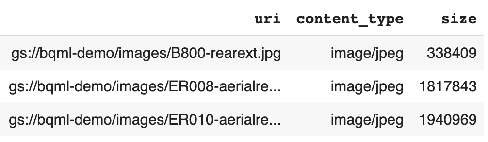
We created the object table, and we're now able to query the object's metadata (and actual data):
SELECT uri, content_type, size
FROM `dataset.demo_images`
LIMIT 3
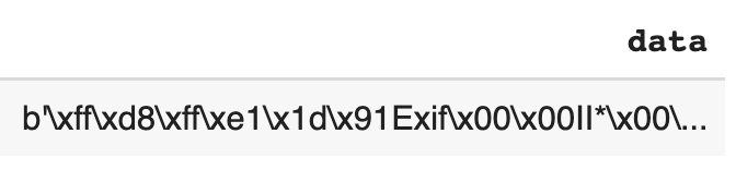
To prove the image data is available, we'll query for it and then render the image with a python function:
SELECT data
FROM `dataset.demo_images`
WHERE REGEXP_CONTAINS(uri, 'B800-rearext.jpg')
Looking at the DataFrame (df) in Pandas we see the bytes of the JPG encoding (notice the Exif):
We can render these bytes as a proper image within a Colab notebook and some helper functions:
from IPython.display import display
from PIL import Image
import io
image = Image.open(io.BytesIO(df.data[0]))
display(image)

There you have it! Images are available directly from BigQuery. Next, we need to run inferences on these images using TensorFlow machine learning models served directly from BQML.
Step 2: Running Inference against BQML TensorFlow Image Models
Saving the Models to BigQuery:
Now it's time to download and serve baseline image models to give us labels and feature vectors. We'll use TensorFlow Hub to search for a good model. We're looking for tried and true image classification and feature vector models. The ResNet 50 models are a good place to start.
> wget -c tfhub.dev/resnet50_etc -O classification.tar.gz
> tar -xf classification.tar.gz --directory classification
To check for compatibility, we'll peek at the model using TensorFlow's saved_model_cli utility:
> saved_model_cli show --dir ./classification --tag_set serve
--signature_def 'serving_default'
Must be in TensorFlow2 format. TensorFlow Lite is not yet supported. The input of the model must:
- Have shape as [batch_size, weight, height, 3] where
- the batch_size must be -1, None, or 1.
- weight, height > 0.
- The input must be dtype = float32 and expect values from [0, 1)
If you have an unsupported model format, you can use TensorFlow + Keras to convert a pre-trained model to a compatible format or fit a custom model with compatible input parameters. A popular technique is applying transfer learning to your specific business domain, starting with a state-of-the-art image model.
Note: Currently, the compressed model must be less than 100 MB and in-memory less than 500 MB.
The ResNet 50 models fit the criteria perfectly. We're ready to upload the models to Cloud Storage and then serve them directly from BQML using the CREATE MODEL statement. We'll use gsutil to upload:
> gsutil -m cp -r ./classification/ gs://bqml-demo/models/
Then we’ll run the CREATE MODEL DDL:
CREATE OR REPLACE MODEL `dataset.resnet50_1k_class`
OPTIONS(
model_type="TENSORFLOW",
color_space="RGB",
model_path="gs://bqml-demo/models/classification/*")
Finally, we're ready for inference!
Running Inference:
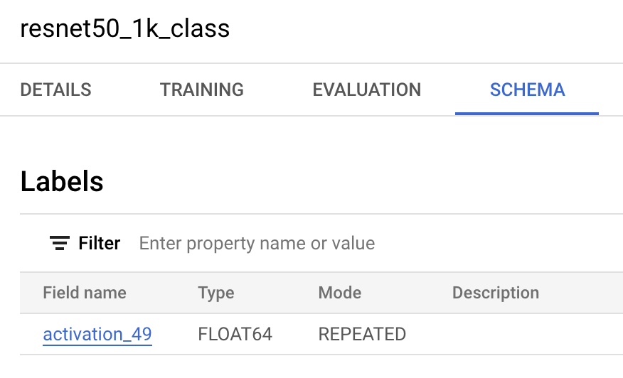
It’s time to drop our images into the served model and get back predictions. You'll need to spend some time structuring your ML.PREDICT() query to your models' specific input and output requirements. In our case, we’ll need to use the output layer of our model, called activation_49, and unnest that array along with the 1,000 labels. You can find the output layer name in your model schema:
We have a few options for moving forward. In this example, we'll use Colab to download the labels into an array and feed that into the ML.PREDICT() statement as a parameterized query:
import urllib.request
label_arr = []
for line in urllib.request.urlopen('https://bit.ly/3SUalN1'):
   label_arr.append(line.decode('utf-8').replace("\n", ""))
_header = label_arr.pop(0)
params = {'labels': label_arr}
Then run the query with IPython Magics, including the params object with the labels:
%%bigquery --params $params
DECLARE labels ARRAY<STRING> DEFAULT @labels;
with predictions as (
 SELECT
   SPLIT(uri, "/")[OFFSET(ARRAY_LENGTH(SPLIT(uri, "/")) - 1)] as img,
   labels[SAFE_OFFSET(i)] as label,
   score
 FROM ML.PREDICT(
     MODEL `bqml-demo.dataset.resnet50_1k_class`,
     (
       SELECT * FROM `bqml-demo.dataset.demo_images`
       LIMIT 1
     )
 ), UNNEST(activation_49) as score WITH OFFSET i
)
SELECT * FROM predictions
ORDER BY score DESC
LIMIT 5;
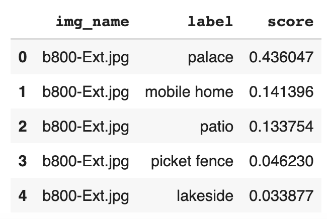
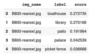
Understanding the output:
To select an image, we’ll need a model to score all the possible image and search combinations. In our simple example, we looked at the labels from the model. In our production pipeline, we take the labels and feature vectors (embeddings) as a step in a larger ML process.
Image editorial is mostly subjective, but the model
can find and learn from patterns in the data.
 |
 |
 |
 |
What stands out to you in this data? Which image would you select? Why? Could we test the decision? Can we trust it? We want the model to be explainable, and with BQML, we have that in Explainable AI. We get access to explainability using ML.GLOBAL_EXPLAIN() and ML.EXPLAIN_PREDICT() functions.
| Overview of Explainable AI ("XAI"): |
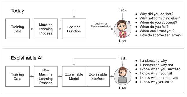 |
| Source: https://www.darpa.mil/program/explainable-artificial-intelligence |
To learn what our CTR prediction model learned, we analyzed the output of ML.GLOBAL_EXPLAIN():
Global Feature Weights for Wide & Deep Vacation Listing Classifier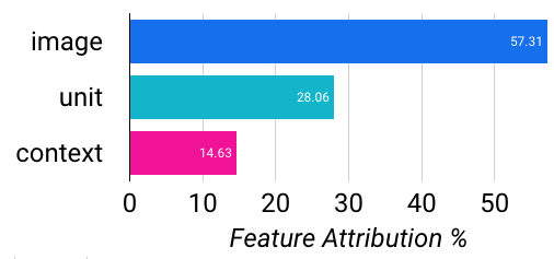 |
These results were fairly shocking. The image fields are sum aggregates of the many features they represent. We had 39 PCA components explaining the 80% of the variance for 2,048 feature vectors. We also took the top five image labels as features. These were fed into our Wide & Deep, among unit and search context features. This model—using vanilla image models, no hyperparameter tuning and default settings—ended up performing quite well:
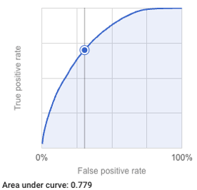
BQML Wide & Deep Vacation Listing Classifier Evaluation
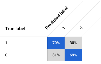 Precision: 0.4198, Recall: 0.7001 Accuracy: 0.6960, F1 score: 0.52 |
 |
We're happy with the result and wanted to share our initial run with no tuning to give you a baseline for your efforts. Note that our tabular features were mainly business and website data.
Step 3: Take Action
In this section, we'll dive into the model output and devise a plan to integrate the predictions into Twiddy's Test and Learn business operations. We want this model to influence two business operations: 1) content editorial—specifically photography and 2) the search appliance experience.
For content editorial, we'll aggregate the predicted click performance by the labels. When we plot that data on a scatter plot, the data tells a story that informs strategy. More pools and beaches; less stairs!
Label Frequency vs. Avg. Probability-to-Click Performance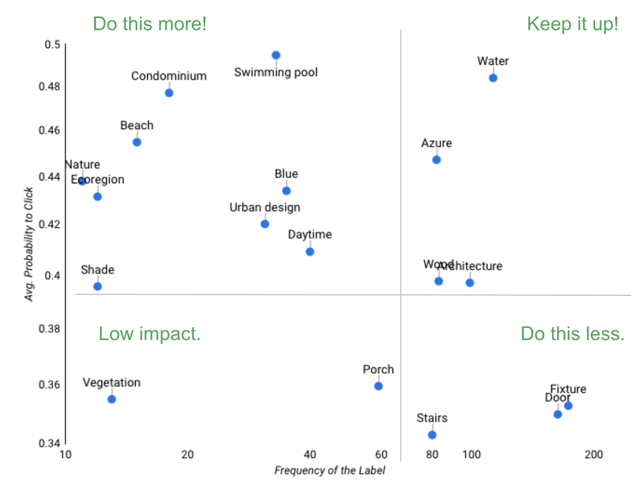 |
| Credit to Google Cloud's "Creative Analysis at Scale" solution for inspiration. |
Secondarily, we want to optimize the search experience. We'll use the predictions to narrow the scope of our A/B test. The model gives us listings with images predicted to perform better. We'll be able to achieve a confidence level for our A/B much faster than cycling through the many hopeless combinations.
Analyzing Predicted Click Performance for Featured Images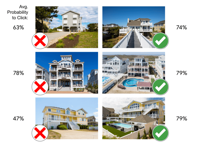 |
| Seed your A/B tests with a strong hypothesis using ML models. This will shorten the time to reach statistical confidence in your tests by removing low-performing candidates from the testing pool. |
Conclusion
Our team enjoyed this project. We got to try out groundbreaking technology from the amazing BQML product team. We got to work with our good friends at Twiddy & Co. Great times all around!
We’re pleased with the result and clearly understand how to use this technology in different domains. Having the pipelines in SQL accelerates our development and maintenance for our clients who typically index higher with SQL skills vs. Python ML experience.
It could be an excellent time to be in the business of developing custom image/audio/video/document models. This technology benefits from transfer learning (aka teaching models about your business), and xfer learning skills are a scarce resource. With inference available in SQL syntax, demand will skyrocket.
The final takeaway is that knowledge of the machine learning process is still critical to delivering business value. While the digitization of tools is a democratizing force, and SQL is one of the most popular languages on the planet, machine learning is about pipelines—a new concept for many analysts. We're excited that these folks will access such a powerful tool. Still, we recognize it will take time and training for the larger analyst community to integrate unstructured data analysis into their day-to-day workflows.
That's a wrap! Please reach out with any questions.