
Share


Those familiar with machine learning (ML) on Google Cloud Platform (GCP) will be proud to tell you there are tons of ML options available that solve different types of problems and for various skill levels, from pre-trained APIs such as Natural Language Processing API to completely custom solutions on AI Platform. But for those of us who work with BigQuery on a daily basis, it’s hard to deny that BQML has brought a lot to the table and it is continuing to
grow
. There is now this general mantra of “you can do ML completely with SQL in BigQuery”. So the idea of this blog post is to explore what end-to-end ML means and how can it be done just with BQML and some SQL and BigQuery magic.
First, what does end-to-end ML mean at its core? Generally, it means two distinct things: we need to have a prediction pipeline and we also need to have a training pipeline. The commonality between the two is that we need a way to trigger them at appropriate times. The need for the prediction pipeline is obvious. We have a trained model and in order to start using it, we need to start making some predictions. Ideally, we’d make those new predictions when new data becomes available.
The training pipeline might be less obvious, and might in some cases depend on the use case, but in most situations, you’d want your model to be retrained periodically to keep it fresh and relevant.
Second, we need to find a use case to implement. At Adswerve we deal with Google Analytics data on a daily basis, and Google Analytics BigQuery export is probably our most loved data source. So what we’ll try to do is predict the likelihood of a user returning to our website within seven days after their session has finished. In other words, users come to our website, browse around for some time and then leave, and the model’s job is to give me a score of how likely they are to return to the website within the next seven days.
Seems cool enough, let’s do it!
 The x-axis values are groups of users grouped by score percentile. So you can see that if you are scored in the top 5% of all sessions (>P95) you are about 95% likely to return, but if you are scored in the bottom 20% of all sessions (<20) you are just about 10% likely to return. The yellow line nicely rises based on the percentile of the score, which is a nice way to validate the model is working as intended.
Beyond model validation visualization, you could actually gain some real insights. For example:
The x-axis values are groups of users grouped by score percentile. So you can see that if you are scored in the top 5% of all sessions (>P95) you are about 95% likely to return, but if you are scored in the bottom 20% of all sessions (<20) you are just about 10% likely to return. The yellow line nicely rises based on the percentile of the score, which is a nice way to validate the model is working as intended.
Beyond model validation visualization, you could actually gain some real insights. For example:
Building a dataset
This is a pretty obvious starting point. We need to write some SQL that will give us a dataset to train against. A dataset should have some quality features and a target to predict. Below is the full SQL used: [sourcecode lang="SQL"] DECLARE lookbackDays DEFAULT 35; -- how far back from the user's last session do we look for activity DECLARE predictionDays DEFAULT 7; -- predicting a user will return in predictionDays days DECLARE currentDate DEFAULT DATE("2020-07-01"); -- we need to align our timezone with GA view's timezone DECLARE startDate DEFAULT DATE_ADD(currentDate, INTERVAL -28*3 DAY); -- taking last 3 months of data WITH user_pool as ( SELECT fullVisitorId, TIMESTAMP_ADD( TIMESTAMP_SECONDS( MAX(visitStartTime) ), INTERVAL -lookbackDays DAY) as lookbackTimestamp FROM `project-id.dataset-id.ga_sessions_*` WHERE SAFE.PARSE_DATE("%Y%m%d", _TABLE_SUFFIX) BETWEEN startDate AND currentDate AND totals.visits IS NOT NULL GROUP BY fullVisitorId ), target AS ( SELECT sessionId, IF( TIMESTAMP_DIFF(nextVisitStartTime, visitStartTime, DAY) &amp;amp;amp;lt;= predictionDays, 1, 0) as label FROM ( SELECT CONCAT(ga.fullVisitorID, visitId) as sessionId, TIMESTAMP_SECONDS( visitStartTime ) as visitStartTime, LEAD( TIMESTAMP_SECONDS( visitStartTime ) ) OVER (PARTITION BY ga.fullVisitorId ORDER BY visitStartTime) as nextVisitStartTime FROM `project-id.dataset-id.ga_sessions_*` as ga INNER JOIN user_pool as up ON up.fullVisitorId = ga.fullVisitorId WHERE SAFE.PARSE_DATE("%Y%m%d", _TABLE_SUFFIX) BETWEEN DATE_ADD(startDate, INTERVAL -lookbackDays DAY) AND DATE_ADD(currentDate, INTERVAL predictionDays DAY) ) ), base AS ( SELECT SAFE.PARSE_DATE("%Y%m%d", _TABLE_SUFFIX) as date, ga.fullVisitorId, clientId, CONCAT(ga.fullVisitorId, visitId) as sessionId, TIMESTAMP_SECONDS(visitStartTime) as visitStartTime, LAG( TIMESTAMP_SECONDS(visitStartTime) ) OVER (PARTITION BY ga.fullVisitorId ORDER BY visitStartTime) as prevVisitStartTime, channelGrouping, ROUND(IFNULL(totals.timeOnSite, 0) / 60, 1) as timeOnSite, IFNULL(totals.pageviews, 0) as pageviews, IFNULL( (SELECT MAX(IF(h.page.pagePath LIKE "/blog/%", 1, 0)) FROM UNNEST(hits) as h WHERE h.type = "PAGE"), 0) as visitedBlogPost, IFNULL( (SELECT MAX(IF(h.page.pagePath LIKE "/our-team/%", 1, 0)) FROM UNNEST(hits) as h WHERE h.type = "PAGE"), 0) as visitedOurTeam, IFNULL( (SELECT MAX(IF(h.page.pagePath LIKE "/services-for-marketers/%", 1, 0)) FROM UNNEST(hits) as h WHERE h.type = "PAGE"), 0) as visitedServices, IFNULL( (SELECT MAX(IF(h.page.pagePath LIKE "/google-marketing-platform/%", 1, 0)) FROM UNNEST(hits) as h WHERE h.type = "PAGE"), 0) as visitedGmp, IFNULL( (SELECT MAX(IF(h.page.pagePath LIKE "/resources/%", 1, 0)) FROM UNNEST(hits) as h WHERE h.type = "PAGE"), 0) as visitedResources, IFNULL( (SELECT MAX(IF(h.page.pagePath LIKE "/forward-together/%", 1, 0)) FROM UNNEST(hits) as h WHERE h.type = "PAGE"), 0) as visitedFwdTogether, IFNULL( (SELECT MAX(IF(h.page.pagePath LIKE "/careers/%", 1, 0)) FROM UNNEST(hits) as h WHERE h.type = "PAGE"), 0) as visitedCareers, IFNULL( (SELECT MAX(IF(h.page.pagePath LIKE "/contact-us/%", 1, 0)) FROM UNNEST(hits) as h WHERE h.type = "PAGE"), 0) as visitedContactUs FROM `project-id.dataset-id.ga_sessions_*` as ga INNER JOIN user_pool as up ON up.fullVisitorId = ga.fullVisitorId AND TIMESTAMP_SECONDS(ga.visitStartTime) &amp;amp;amp;gt;= up.lookbackTimestamp WHERE SAFE.PARSE_DATE("%Y%m%d", _TABLE_SUFFIX) BETWEEN DATE_ADD(startDate, INTERVAL -lookbackDays DAY) and currentDate ), dataset as ( SELECT * EXCEPT(label, prevVisitDaysAgo, avgDaysBetweenVisits, ttlVisitedBlogPost, ttlVisitedOurTeam, ttlVisitedServices, ttlVisitedGmp, ttlVisitedFwdTogether, ttlVisitedCareers, ttlVisitedContactUs ), ML.BUCKETIZE(prevVisitDaysAgo, [2, 4, 7, 14, 21, 28]) AS prevVisitDaysAgo, ML.BUCKETIZE(avgDaysBetweenVisits, [2, 4, 7, 14, 21, 28]) AS avgDaysBetweenVisits, ROUND(ttlVisitedBlogPost / sessions, 2) as visitedBlogPostPerSession, ROUND(ttlVisitedOurTeam / sessions, 2) as visitedOurTeamPerSession, ROUND(ttlVisitedServices / sessions, 2) as visitedServicesPerSession, ROUND(ttlVisitedGmp / sessions, 2) as visitedGmpPerSession, ROUND(ttlVisitedFwdTogether / sessions, 2) as visitedFwdTogetherPerSession, ROUND(ttlVisitedCareers / sessions, 2) as visitedCareersPerSession, ROUND(ttlVisitedContactUs / sessions, 2) as visitedContactUsPerSession, label FROM ( SELECT date, fullVisitorId, clientId, t.sessionId, visitStartTime, -- row not to be used in training ROUND( COS(ACOS(-1) * (EXTRACT(DAYOFWEEK FROM visitStartTime)-1 + EXTRACT(HOUR FROM visitStartTime)/24) / 3.5), 2) AS weekdayx, ROUND( SIN(ACOS(-1) * (EXTRACT(DAYOFWEEK FROM visitStartTime)-1 + EXTRACT(HOUR FROM visitStartTime)/24) / 3.5), 2) AS weekdayy, channelGrouping, COUNT(*) OVER (PARTITION BY fullVisitorId ORDER BY visitStartTime) as sessions, IFNULL(ROUND( TIMESTAMP_DIFF(visitStartTime, prevVisitStartTime, HOUR) / 24, 1), lookbackDays) as prevVisitDaysAgo, IFNULL(ROUND( AVG( TIMESTAMP_DIFF(visitStartTime, prevVisitStartTime, HOUR) ) OVER (PARTITION BY fullVisitorId ORDER BY visitStartTime) / 24, 1), lookbackDays) as avgDaysBetweenVisits, timeOnSite as currentTimeOnSite, ROUND( AVG( timeOnSite ) OVER (PARTITION BY fullVisitorId ORDER BY visitStartTime), 1) as avgTimeOnSite, visitedBlogPost, visitedOurTeam, visitedServices, visitedGmp, visitedFwdTogether, visitedCareers, visitedContactUs, SUM( visitedBlogPost ) OVER (PARTITION BY fullVisitorId ORDER BY visitStartTime) as ttlVisitedBlogPost, SUM( visitedOurTeam ) OVER (PARTITION BY fullVisitorId ORDER BY visitStartTime) as ttlVisitedOurTeam, SUM( visitedServices ) OVER (PARTITION BY fullVisitorId ORDER BY visitStartTime) as ttlVisitedServices, SUM( visitedGmp ) OVER (PARTITION BY fullVisitorId ORDER BY visitStartTime) as ttlVisitedGmp, SUM( visitedFwdTogether ) OVER (PARTITION BY fullVisitorId ORDER BY visitStartTime) as ttlVisitedFwdTogether, SUM( visitedCareers ) OVER (PARTITION BY fullVisitorId ORDER BY visitStartTime) as ttlVisitedCareers, SUM( visitedContactUs ) OVER (PARTITION BY fullVisitorId ORDER BY visitStartTime) as ttlVisitedContactUs, t.label FROM base INNER JOIN target as t ON t.sessionId = base.sessionId ) ) SELECT * FROM dataset; [/sourcecode] While the SQL is on the long side, it’s a nice trade-off between a toy example and a full-on feature engineered dataset. One thing worth mentioning is that we will be using BigQuery scripting in this blog post, which you can see in the DECLARE statements in the above query, but it will get a bit more intense later on. With the dataset query done, we have something to train on, but what about at prediction time? Will we need another query to construct a prediction dataset? Well, not necessarily, and likely it’s best if we make sure we keep things as consistent as possible. As it is well known, the way we construct the training dataset must also be the way we construct the prediction dataset. So why not package them into one unit? Here’s how. Let’s use BigQuery stored procedures so our dataset creation SQL is nicely tucked into a single unit of execution, which we can control with some input parameters: [sourcecode lang="sql"] CREATE OR REPLACE PROCEDURE `project-id.bq_mlpipeline.create_dataset`(currentDate DATE, startDate DATE, lookbackDays INT64, predictionDays INT64, mode STRING) BEGIN CREATE TEMP TABLE temp_dataset AS dataset query IF mode = "train" THEN CREATE OR REPLACE TABLE `bq_mlpipeline.dataset_train` OPTIONS( expiration_timestamp=TIMESTAMP_ADD(CURRENT_TIMESTAMP(), INTERVAL 1 DAY) ) AS SELECT * EXCEPT(date, fullVisitorId, clientId, sessionId, visitStartTime) FROM temp_dataset; ELSEIF mode = "predict" THEN CREATE OR REPLACE TABLE `bq_mlpipeline.dataset_prediction` OPTIONS( expiration_timestamp=TIMESTAMP_ADD(CURRENT_TIMESTAMP(), INTERVAL 1 DAY) ) AS SELECT * EXCEPT(label) FROM temp_dataset WHERE date BETWEEN startDate AND currentDate; END IF ; DROP TABLE temp_dataset; END ; [/sourcecode] To break this down just a little, at the top we have our dataset query that is wrapped up in a CREATE TEMP TABLE statement that allows us to later refer to the result just like you would refer to a normal table, except the temp table lives just inside the stored procedure and the query, once executed, doesn’t have to be executed again when you are referring to it. The part after that is a bit more interesting. We have an IF statement, with one branch taking care of the training dataset and the other for prediction dataset. Namely, the train part does not need some of the “metadata” fields in the dataset such as fullVisitorId, and on the opposite side, the prediction part does not need to know about the label. It’s very easy to call this procedure with the parameters you want, knowing it will construct the dataset correctly for both training or prediction dataset with one core query inside: [sourcecode lang="sql"] CALL bq_mlpipeline.create_dataset( currentDate, startDate, lookbackDays, predictionDays, '<train|predict>' ); [/sourcecode]Building a training pipeline
After we successfully create the dataset, we need to train the model and do some Exploratory Data Analysis (EDA) and such to make sure we get the best performance. Let’s assume we’ve done that already and it’s time to make sure our model gets retrained on some cadence. We already have all the building blocks, but we now need BigQuery Scheduled Queries. If you are not aware of what that is you can start here . Our training query ends up being pretty simple: [sourcecode lang="sql"] DECLARE lookbackDays DEFAULT 35; -- how far back from the user's last session do we look for activity DECLARE predictionDays DEFAULT 7; -- predicting a user will return in predictionDays days DECLARE currentDate DEFAULT DATE_ADD(DATE(@run_time, "America/Denver"), INTERVAL -predictionDays DAY); -- we need to align our timezone with GA view's timezone DECLARE startDate DEFAULT DATE_ADD(currentDate, INTERVAL -28*3 DAY); -- taking last 3 months of data CALL bq_mlpipeline.create_dataset( currentDate, startDate, lookbackDays, predictionDays, 'train' ); CREATE OR REPLACE MODEL `bq_mlpipeline.model` OPTIONS( MODEL_TYPE='LOGISTIC_REG', --AUTO_CLASS_WEIGHTS=TRUE, L2_REG=0.75, LS_INIT_LEARN_RATE=0.5, MIN_REL_PROGRESS=0.001 ) AS SELECT * FROM `bq_mlpipeline.dataset_train` [/sourcecode] The only thing worth mentioning here is the @run_time parameter that’s coming from the scheduled query service and tells us the current timestamp of the execution. Based on this timestamp, we can adjust the start and end dates of the training dataset. After that, we call our stored procedure and finally we train the model. In our case, we scheduled this to run the first day of every month and the model will be replaced each month with a newer version.Building the prediction pipeline
The key question here is when the new data becomes available. With the GA export to BQ the answers may vary, but the most straightforward one is that new data becomes available each day for the previous day. Meaning you are always one day behind. There are also intraday tables that update about every few hours during the day. This is better as you no longer need to wait a full day to get to some new predictions. There’s also the realtime export which lags about five to 15 minutes, so that’s even better. While there are many possibilities for different use cases, we’ll stay with the most straightforward one and assume new data comes each day. With scheduled queries at our disposal, we’re good to go. We just need to answer two more questions: when do we set our schedule query to run and when will the new table be available? This can be tricky and can vary from day to day as there is no set time when the data should appear. We’re in the classic situation where we don't want to wait too long to get the predictions, but also we don’t want to schedule it too early and end up with no new predictions. We can use some SQL scripting and do it “the middle way”. We can schedule our query to run every hour and first check if the data is available and only then do the prediction, but only if the prediction hasn’t been made today. Here’s how: [sourcecode lang="sql"]</pre> DECLARE currentDate DEFAULT DATE(@run_time, "America/Denver"); -- we need to align our timezone WITH GA view's timezone -- actual prediction date is one day before currentDate because ga_sessions daily table is created for yesterday DECLARE predictionDate DEFAULT DATE_ADD(currentDate, INTERVAL -1 DAY); DECLARE startDate DEFAULT predictionDate; -- DATE_ADD(currentDate, INTERVAL -28*3 DAY); DECLARE lookbackDays DEFAULT 35; DECLARE predictionDays DEFAULT 7; DECLARE predictionTableName DEFAULT "predictions"; -- this will hold info if a new GA dail table exists DECLARE existsGaSessions BOOL; -- this will hold info if our predictions table exists (it should only not exist on the first run) DECLARE existsPredictionTable BOOL; -- this will hold info if our prediction process already ran for today, so no need to run again DECLARE alreadyRanToday BOOL; # START: GA SESSIONS TABLE EXISTENCE CHECK -- first we need to check if our source table exists SET existsGaSessions = ( SELECT COUNT(*) > 0 FROM `analyticspros.com:spotted-cinnamon-834.24973611.INFORMATION_SCHEMA.TABLES` WHERE table_name = CONCAT("ga_sessions_", FORMAT_DATE("%Y%m%d", predictionDate)) ); -- if ga_sessions doesn't exists yet, just leave there is nothing to do IF NOT existsGaSessions THEN RETURN; END IF ; # END: GA SESSIONS TABLE EXISTENCE CHECK # START: PREDICTION TABLE EXISTENCE CHECK SET existsPredictionTable = ( SELECT COUNT(*) > 0 FROM `bq_mlpipeline.INFORMATION_SCHEMA.TABLES` WHERE table_name = predictionTableName ); IF NOT existsPredictionTable THEN -- create a table to run predictions on CALL bq_mlpipeline.create_dataset( predictionDate, startDate, lookbackDays, predictionDays, 'predict' ); -- run predictions and create the new table CREATE TABLE `bq_mlpipeline.predictions` PARTITION BY date CLUSTER BY sessions AS SELECT date, fullVisitorId, clientId, sessionId, visitStartTime, sessions, (SELECT p.prob FROM UNNEST(predicted_label_probs) as p WHERE p.label = 1) as prediction FROM ML.PREDICT(MODEL `bq_mlpipeline.model`, TABLE `bq_mlpipeline.dataset_prediction`); RETURN; END IF; # END: PREDICTION TABLE EXISTENCE CHECK # START: ARE WE ALREADY DONE FOR TODAY SET alreadyRanToday = ( SELECT COUNT(*) > 0 FROM `bq_mlpipeline.predictions` WHERE date = predictionDate ); IF NOT alreadyRanToday THEN -- create a table to run predictions on CALL bq_mlpipeline.create_dataset( predictionDate, startDate, lookbackDays, predictionDays, 'predict' ); INSERT INTO `bq_mlpipeline.predictions` SELECT date, fullVisitorId, clientId, sessionId, visitStartTime, sessions, (SELECT p.prob FROM UNNEST(predicted_label_probs) as p WHERE p.label = 1) as prediction FROM ML.PREDICT(MODEL `bq_mlpipeline.model`, TABLE `bq_mlpipeline.dataset_prediction`); RETURN; END IF; # END: ARE WE ALREADY DONE FOR TODAY [/sourcecode] Hopefully, the query has enough comments to guide you through. We can schedule the above query to run every hour and so we don’t risk scheduling too early or too late, but instead periodically check.Thoughts on the solution
I believe we can truly say end-to-end ML is possible without ever leaving BigQuery or even using anything other than SQL. This solution is great for POC projects where you can show the value of the model extremely fast. There are some shortcomings as well. For example, storing previously trained models in case the current retrain goes bad. Instead of triggering the prediction pipeline on a schedule, one could trigger it in an event-based way. Email notifications with retrained stats would be great or just error emails in general, to name a few. However, all of the shortcomings still do not overshadow the fast development BQ offers in this case. We focused on the GA export data only, but you could also include other datasets that would bring in valuable features such as CRM or CMS data. Or you could even bring in data from Ads Data Hub to create aggregated features around paid media exposures.Visualizing the model
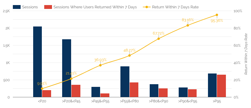
With all of the above in place, you can visualize the model to get a better idea of the performance and to monitor the predictions over time.
The x-axis values are groups of users grouped by score percentile. So you can see that if you are scored in the top 5% of all sessions (>P95) you are about 95% likely to return, but if you are scored in the bottom 20% of all sessions (<20) you are just about 10% likely to return. The yellow line nicely rises based on the percentile of the score, which is a nice way to validate the model is working as intended.
Beyond model validation visualization, you could actually gain some real insights. For example:
- Per percentile group, visualize features such as time on site, sessions per user, pageviews, etc. to be able to see how core features differ per group
- Per percentile group, visualize what channels bring in users with the best scores. This can help you determine what channels are better drivers of user retention
- Per percentile group, visualize content visits. This allows you to see what content your top users are seeing vs your low-value users